
This guest blog post is part of a series on loop tuning. This blog post is Part 1 in the loop tuning series. Click these links to read Part 2 and Part 3.
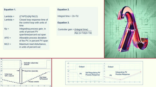
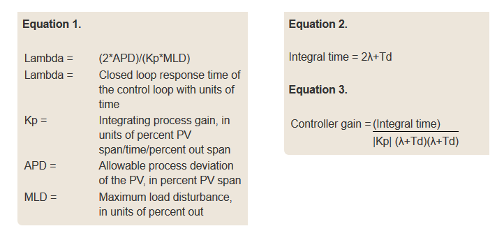
The two most common categories of process responses in industrial manufacturing processes are self-regulating and integrating. A self-regulating process response to a step input change is characterized by a change of the process variable, which moves to and stabilizes (or self-regulates) at a new value. An integrating process response to a step input change is characterized by a change in the slope of the process variable.
From the standpoint of a proportional, integral, derivative (PID) process controller, the output of the PID controller is an input to the process. The output of the process, the process variable (PV), is the input to the PID controller.
Level processes typically have an integrating response, the likely exception being when the outflow of the vessel is gravity driven. Other processes can have an integrating response. For example, a “low-pressure, large-volume” gas pressure control application can have an integrating process. Another example of an integrating process is a reactor temperature controller that cascades to a “jacket water inlet temperature difference” controller. This controller controls the difference between the reactor contents’ temperature and the jacket water inlet’s temperature based on the set point specified by the output of the reactor contents’ temperature controller.
Challenges
One of the challenges of tuning a PID controller for an integrating process is that when the integral action of the controller is combined with the integrator function of the process, the control loop will oscillate if the integral action of the controller is “too fast” (i.e., the integral time is too short). It is not intuitive to know when the integral time is too short. Another challenge is that most PID tuning methods for integrating processes do not provide a method to adjust the aggressiveness of the closed loop response. If the controller proportional gain (P) is reduced to make the closed loop response less aggressive, the loop is more likely to oscillate. This is quite the opposite result of when this tactic is used on a self-regulating process.
Tuning for an integrating process
A tuning methodology called lambda tuning solves these challenges. The lambda tuning method allows the user to choose the closed loop response time, called lambda, and calculate the corresponding tuning. The lambda closed loop response time is chosen to achieve the desired process goals and stability criteria. This could result in choosing a small lambda for good load regulation, a large lambda to minimize changes in the controller output and manipulated variable by allowing the PV to deviate from the set point, or somewhere in between these two extremes. Lambda tuning for integrating processes results in tuning that produces a “critically damped,” nonoscillatory response for a step load or set point change (i.e., some oscillation when lambda is less than three times dead time).
Procedure
The lambda tuning method for integrating processes involves three steps:
- Identify the process dynamics.
- Choose the desired closed loop speed of response, lambda.
- Calculate the required PID tuning constants.
Figure 3 (see InTech article) shows the dynamic parameters of an integrating process. The dynamic parameters that describe the integrating response are dead time (Td), in units of time, and the integrating process gain (Kp), in units of percent PV span/time unit/percent output span. Note that the process variable can have a nonzero initial slope when performing the step test to measure the process dynamics.
This blog post is Part 1 in the loop tuning series. Click these links to read Part 2 and Part 3.
Typically several step tests are performed; the results are reviewed for consistency; and the average process dynamics are calculated and used for the tuning parameter calculations. If the controller output goes directly to a control valve, any significant dead band in the valve will cause reduced process gain if the output step was a reversal in direction. If the controller output cascades to the set-point point of a “slave” loop, the slave loop should be tuned first.
The next step is to choose the lambda to achieve the desired process control goal for the loop. If the goal is the best load regulation, choose a shorter lambda. If the goal is to absorb variability in the vessel by allowing the level to vary and lessen the movement of the controller output and manipulated variable, then choose a longer lambda. A shorter lambda produces more aggressive tuning and less stability margin. A longer lambda produces less aggressive tuning and more stability margin. The low limit on lambda for an integrating plus dead time process (no lag or lead in the response) is equal to the dead time, although this provides a very low gain margin and phase margin. A more reasonable low limit on lambda is three times the dead time. Care should be taken to make sure the dead time does not increase under any other conditions if the lambda is set equal to the dead time. From a stability standpoint, there is no upper limit on the lambda. However, the lambda must be fast enough to keep the process variable within the allowable process deviation (APD) for the maximum load disturbance (MLD). The required lambda can be estimated with equation 1, subject to the minimum limit on lambda. Note that the time units of lambda will be the same as the time units used for the integrating process gain, Kp.
This formula can be used regardless of whether “tight” control is desired, to provide good load regulation, or “averaging” control is desired, to reduce variability of the manipulated variable by reducing the controller output movement.
The final step is to calculate the tuning parameters from the process dynamics. Care should be taken to use consistent units of time for the integrating process gain, the dead time, and the lambda. For a pure integrator plus dead time process (no significant lag or lead), the controller gain and reset times are calculated with the following equations. The derivative time is set to 0. These equations are valid for the standard (sometimes called ideal, noninteractive) and series (sometimes called classical, interactive) forms of the PID implementation. Note that both the controller gain and integral time change as lambda (λ) changes.
Example
Consider the distillation column feed storage tank level control process in figure 4 (see InTech article). The level controller, LIC-1, output is cascaded to the set point of the column feed flow controller, FIC-2. FIC-2 has been properly tuning and responds in a nonoscillatory manner with a closed loop response time, lambda, of 6 seconds. It is desirable to minimize the changes in the column feed rate by using the capacity of the feed tank to attenuate the transfer of the variability of the reactor flows into the tank to the flow out of the tank, which is the feed flow to the distillation column.
Figure 5 (see InTech article) shows a step test of the level controller to identify the process dynamics. The integrating process gain is –0.000216 percent level/second/percent out, and the dead time is about 30 seconds. Based on the process goals, the APD selected for the level PV is 30 percent. It is often appropriate in these applications to use a fraction of the nominal controller output as the MLD. The idea is to find the MLD for which the controller is expected to keep the PV within the APD without operator intervention. Load changes larger than the chosen MLD are expected to require operator intervention due to other consequences. After reviewing the process, the maximum load disturbance is chosen to be 50 percent of the nominal 80 percent controller output, or 40 percent. This represents the loss of two reactors simultaneously. The required lambda and the resulting tuning parameters using the lambda tuning method are calculated from equations 1, 2, and 3, respectively. These values are shown below.
Lambda = 6,900 seconds
Integral time = 13,830 seconds
Controller gain = 1.34
Simulation of the process response to a step load disturbance equal to 40 percent controller output (MLD) confirms that the recommended tuning will keep the level deviation (APD) to less than ±30 percent and that the response is nonoscillatory. The calculated tuning was installed in the level controller, and the system performed as desired.
Meeting process goals
Tuning PID controllers for integrating or near-integrating processes is counterintuitive when compared to tuning for self-regulating processes. Most published PID controller tuning methods for integrating processes are designed for optimum load rejection, not necessarily optimum process performance. The lambda tuning method provides the ability to tune the PID controller to achieve process performance goals, whether they are maximum load regulation or attenuation of variability.
A version of this article also was published at InTech magazine.


